This page guides you through first steps with Met.3D after you have installed the software. Please also refer to the slides at Slides: Introductory Met.3D tutorial.
Note: The screenshots on this page may be taken with different versions of Met.3D. You may observe small changes in the user interface in the current version you are using.
Starting Met.3D
For the first steps with Met.3D, simply start the software by calling
$ ./met3D
You will see some debug and info output on the console. Fig. 1 shows the Met.3D window that appears on first start-up. It contains an empty visualization area.
 Met.3D main window that appears when first starting the software.")
Fig. 1: The (empty) Met.3D main window that appears when first starting the software.
Adding actors to a scene
Next, add first visualization objects to the empty visualization area. In Met.3D, visualization objects are called actors. Actors represent, for example, a graticule, a base map, a 2D horizontal or vertical cross-section, or 3D isosurfaces. Currently available actors are listed in Visualization objects ("Actors"). Actors are grouped into scenes, which are simply a collection of actors. A single actor can be assigned to one or to multiple scenes. A scene can be visualized by one or by multiple scene views, which are the visualization areas in the Met.3D window. In Fig. 1, one scene view (“view 1”) is visible. It displays “Scene 1”, which currently does not contain any actors. To add actors to this scene, follow these steps:
- Select the menu entry “View/Scene Management” (or press “F4”) to open the scene management dialog displayed in Fig. 2. The dialog shows available scenes on the right hand side, and available actors on the left (the listed “Labels” actor corresponds to a special system actor that is always present and that is responsible for text rendering). The buttons below the list of actors provide functionality to create new default actors, to load actor configurations from file, and to delete existing actors.

Fig. 2 The scene management dialog. Open with “View/Scene Management” or by pressing “F4”. - First, create a new (default) graticule actor. Click on the “create” button in the “Actor settings” section. In the dialog that appears, select “Graticule” and name the actor correspondingly.
- Next, add the graticule actor to “Scene 1”. To do this, select the actor in the list of actors, then check the scenes in which it should appear in the list of scenes below (Fig. 3). When you click on “Scene 1”, the graticule will appear in the Met.3D window in the background.

Fig. 3 After the new default graticule actor has been created, it can be assigned to “Scene 1” by selecting the actor and checking the corresponding scene(s). - Repeat the steps for a volume bounding box actor and a base map actor.
- Close the dialog. Your Met.3D window now looks like Fig. 4. The base map is black, as no map has been loaded yet. To load a map, the actor needs to be configured. On the left hand side of the Met.3D window, below the navigation controls for time and ensemble member, the “Scene 1” tab lists the actors that are assigned to the scene. It provides access to the actors’ properties. The properties are organised in a tree structure (in the following called “property tree”) and grouped into different categories, depending on their function.

Fig. 4 The Met.3D main window after graticule, volume bounding box and base map have been added. No base map file has been loaded yet, hence the map appears black. - Open the property tree for the base map actor. In the “actor properties” group, find the “load map file” entry. Click on the button to open a file dialog.
- Choose the raster base map that you have downloaded from Natural Earth (see installation) and confirm. After the file has been loaded, your Met.3D window looks like Fig. 5.

Fig. 5 The same as Fig. Fig. 4 with a base map file loaded. The configured base map actor can be saved to an actor configuration file, so that the configuration steps do not have to be repeated each time a base map actor is required (this is particularly important if more properties than just the path to a map file have to be set for a given actor). In the base map actor’s “configuration” group, select the “save” entry. For example, create a new subdirectory
~/met3d/actors/in your Met.3D home directory (see installation), and store the configuration tobasemap_default.actor.conf. All actor configuration files need to end with.actor.conf.To check whether the configuration has been stored successfully, open the scene management dialog again. Select the base map actor in the list of actors in the “Actor settings” section and click “remove”. Next, click “create from file” and select the file that you have just stored. The actor reappears in the list and can be reassigned to “Scene 1”.
Working with scenes and scene views
Met.3D provides standard mouse interaction techniques to change the observer’s point of view within a scene view. Hold the left mouse button and drag to rotate the scene, the right button to pan, and use the scroll wheel to zoom.
Many default settings of the user interface can be changed by using customized configuration files for the Met.3D "frontend". For example, a frontend configuration file can be passed on the command line:
$ ./met3D --frontend=~/met3d/config/frontend.cfg
An an example, the default mouse interaction for navigation can be changed in the [SceneNavigation] section of a custom frontend.cfg. Simply copy the default_frontend.cfg file from the met.3d-base/met.3d/config/ subdirectory to the location of your choice, edit, and pass the file on the command line as done above.
See the default file provided with Met.3D for further examples:
The number and layout of displayed scene views can be changed by selecting one of the presets in the “View” menu (the preset configurations in the menu are also available through the keyboard short-cuts Alt+0..6). The default maximum number of scene views is four. For example, Fig. 6 shows the layout “one large view and three small views” (Alt+5).

Fig. 6 Met.3D window layout with one large and three small scene views. Views 1, 2 and 3 all show “Scene 1”, but from different viewpoints.
Similar to actor configurations, viewpoints (camera positions) can be saved to file and restored at a later time. To save a given viewpoint, select the “System” tab on the left of the Met.3D window. Similar to actor properties, properties affecting the scene views are arranged in a property tree. Open the property for the scene view for which you would like to save the camera, and choose the “modify camera/save” property.
Multiple scene views can show the same scene. In the example in Fig. 6, views 1, 2 and 3 all show “Scene 1”, but from different viewpoints. To achieve this, open the scene management dialog and specify the scenes that the views display in the lower left area of the dialog (cf. Fig. 2). Also, in view 3 the vertical scaling of the scene is different to views 1 and 2. The vertical scaling can also be changed in the “System” tab on the left side of the Met.3D window. As an example, modify the “rendering/vertical scaling” parameter for view 1 and observe the difference. With “interaction/sync camera with view”, it is possible to synchronize the camera viewpoints of two scenes. This is useful if two different scenes are to be examined from the same viewpoint.
Actors can be assigned to multiple scenes by selecting the corresponding scenes in the scene management dialog (Fig. 3). This way, actors such as graticule, base map or volume bounding box can be shared among different scenes (representing “static” content) and combined with different forecast actors (“dynamic” content) in the individual scenes.
For actors that allow interaction with the user, the scene views provide an “interaction mode”. The interaction mode can be enabled by pressing “i” while a scene view is selected, by double-clicking in the view, or by checking the corresponding property in the scene view’s property tree. While the interaction mode is enabled for a scene view, the text “Interaction mode” appears at the bottom of the view and the camera is frozen.
As an example, the “movable poles” actor supports user interaction. It allows the user to move a pole within the scene by dragging a handle attached to a pole. The following steps add the actor to the current configuration:
- In the scene management dialog, create a new instance of the “movable poles” actor and add the instance to “Scene 1”. As no specific pole has been defined yet, there is nothing to see so far.
- In the actor’s property tree, the “actor properties” group contains the entry “add pole”. Click on the button to create a new pole. By default, it is placed at (lon/lat) = (0/0). Enter “Y=45” to manually specify the latitude. The pole is now located in western France. Fig. 7 shows the corresponding Met.3D window (note that the “one large, two small views” layout was activated by pressing Alt+4).

Fig. 7 Met.3D window with a movable pole. - Click on the large scene view (“view 1”) and press “i” (or double-click) to activate the interaction mode. Now, small spheres that act as handles appear at the top and bottom of the pole. Move the mouse pointer over the bottom handle of the pole. The handles are now highlighted in red (Fig. 8).

Fig. 8 Met.3D window with a movable pole, in interaction mode. - Click on the handle and drag the pole. Note how the pole’s position is updated in all scene views that display the scene.
Adding actors that visualize gridded simulation data to the scene
Next, we add a horizontal cross-section that displays some gridded simulation data (e.g., of a numerical weather prediction). The goal is to create a forecast product that shows colour-coded wind speed, overlain with contour lines of geopotential height and wind barbs.
Configuring a data pipeline (adding a dataset)
Met.3D uses the notion of a data pipeline to access gridded data, e.g. those from a numerical weather prediction model. A data pipeline realizes access to a dataset that can contain multiple simulation variables, time steps, ensemble members, etc., in a single or in multiple files in NetCDF or GRIB format. Supported file types and grid types are described in more detail in Data handling.
Data pipelines can be created at runtime or in a configuration file and loaded on start-up of the software. Here we use the simple option to load a dataset at runtime: Select "Add new dataset" from the "File" menu, and fill in the necessary fields in the dialog that appears.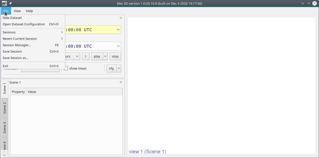
TODO: Add screenshot and description of GUI interface.
Adding a horizontal section
We assume the dataset being registered with the data source identification ECMWF ENS EUR_LL10.
- In the scene management dialog, create a “horizontal cross-section”. Add the section to the current scene.
- To map the wind speed data to colour, a transfer function (i.e. a colour map) is required. Create and add a “1D transfer function” and close the scene management dialog. The Met.3D window now looks like Fig. 9 (where the default settings of colour bar and section may vary depending on the exact Met.3D version). The horizontal section by default contains an instance of a graticule actor that replicates the graticule and coast lines at the elevation of the section.

Fig. 9 An empty horizontal section and a colour bar (1D transfer function) have been added to the scene. - All actors that display forecast data make use of “variables” that represent a given forecast parameter (e.g. wind speed) and store the actor-related settings that correspond to this parameter. For example, in the case of a horizontal section, these settings include whether the parameter shall be visualized as line contours or as filled contours and, in the latter case, which colour map shall be used. To add a variable to the horizontal section, select “add new variable” in the actor’s “variables” group in the property tree. The dialog that opens is shown in Fig. 10. It lists all available forecast parameters that are available from the registered data sources.

Fig. 10 Data source selection dialog. The dialog lists all forecast parameters that are available from the registered data pipelines. - From the list, select the data source
ECMWF ENS EUR_LL10 ENSFilterand the variableWindspeed_hybrid. The suffix “ENSFilter” in the data source name indicates that in the data pipeline, a module that computes statistical quantities from the ensemble (e.g. mean or standard deviation) has been attached to the original dataset. Confirm the forecast parameter selection. In the follow-up dialog about a synchronization control select “Synchronization” to synchronize the variable with the global time and ensemble settings. - The variable appears in the property tree of the horizontal section actor. In the variable’s subgroup “rendering”, find the properties “transfer function” and “render mode”. Select the transfer function that you have created above and set the render mode to “filled contours”. The scene now looks like the screenshot in Fig. 11.

Fig. 11 A variable containing horizontal wind speed has been added to the horizontal section. The colour bar (1D transfer function) has been connected to the variable. - Next, the colour map needs to be adjusted. Open the property tree of the colour map. In the “actor properties/range” subgroup, set “decimals” to 0 and the minimum and maximum value to 10 and 80, respectively. The colour map type is set to “predefined” (vs. HCL, see 1D transfer function (Colour map)). Open the “predefined” group and select “hot_wind”. Also check the “reverse” field. Now, the horizontal sections displays the wind speed as shown in Fig. 12.

Fig. 12 Modification of the colour map to reflect the range of values in the wind speed variable. - Go back to the horizontal section actor’s property tree and add a second variable. This time, choose
Geopotential_height_hybrid. For this variable, we set “render mode” to “line contours”. Potential contour values can be specified in the text fields “thin contour levels” and “thick contour levels”. The strings can either be a list of values (e.g.5000,5500,6000) or three values of format[from,to,step]. An example of the latter is[0,26000,40], which will display a contour line every 40 m between 0 and 26000 m. Note that the range of values is chosen to reflect all possible values that might be encountered at any vertical location of the section. Met.3D will recognize which of the values are applicable to a given elevation and only render the actually visible lines. Put[0,26000,40]into the “thin contour levels” field and[0,26000,200]into the “thick contour levels” field. The result is shown in Fig. 13.
Fig. 13 Contour lines of geopotential height have been added to the section. - To complete the forecast product, add two more variables to the actor:
u-component_of_wind_hybridandv-component_of_wind_hybrid. Leave the “render mode” for both variables set to “disabled”. Instead, open the “actor properties/wind barbs” property group of the horizontal section actor. At the bottom of the group, assign the u and v-components to the corresponding fields and click on “enabled”. For the screenshot in Fig. 14, I have also changed the colour of the barbs to blue.
Fig. 14 Wind barbs have been added to the section.
The forecast product has been completed. Switch to actor interaction mode (double click in the scene view) to drag the section up and down, or modify the “actor properties/slice position” property, and use the time and ensemble navigation buttons in the top left of the Met.3D window to change time and/or ensemble member. Of course, the horizontal section configuration can be saved to a configuration file, a saved horizontal section actor configuration can be loaded at runtime in the scene management dialog. Alternatively, it can be listed in the frontend.cfg file to be loaded during start-up.
You can also have multiple instances of an actor in a scene. Fig. 15 shows an example of two horizontal sections stacked on top of each other (the lower one at 925 hPa and the upper one at 200 hPa). The pole is placed in the centre of the low pressure system at 925 hPa, its intersection with the upper section showing the relation of the position of low-level centre to the jet stream.

Fig. 15 Two identical horizontal sections stacked on top of each other. The vertical pole illustrates the relation between low pressure centre at 925 hPa and the jet stream at 200 hPa.